iPheGWAS - Bringing intelligence to an improved PheGWAS
iphegwas.RmdiPheGWAS (intelligent -PheGWAS) module is developed to bring intelligence into PheGWAS by incorporating a new heuristic approach developed by our team to order traits based on its genetic correlation quickly and efficiently. As a result, the iPheGWAS module is integrated seamlessly into the PheGWAS module. We also improved the previous PheGWAS codebase for faster landscape visualization.
This package is packaged with datasets used in PheGWAS and some datasets to demonstrate iPheGWAS and from the paper. If you are looking for the entire data used for studies 1 and 2 in iPheGWAS, please download it from here. Checkout the individual datasets here.
Here are the datasets that are available from iPheGWAS study2 within the package.
- ibd
- Wasisthipratio
- CrohnsDisease
- UlcerativeColitis
- bmi
Loading iphegwas package;
library(iphegwas)Using iphegwas module
Your GWAS summarystats file/dataframe should have columns named in this way.
CHR BP rsid A1 A2 beta se P.valueYou can fun iPheGWAS in 2 modes, - Mode 1: Folder path to the summary statistics file. - Mode 2: Passing the dataframe names available in your environment to iphegwas module as vector of dataframe names.
Mode 1
## Giving absolute file path pathname <- '<path to your folder>'
pathname <- system.file("extdata", "samplesummary", package = "iphegwas")
iphegwas(pathname = pathname, dentogram = TRUE)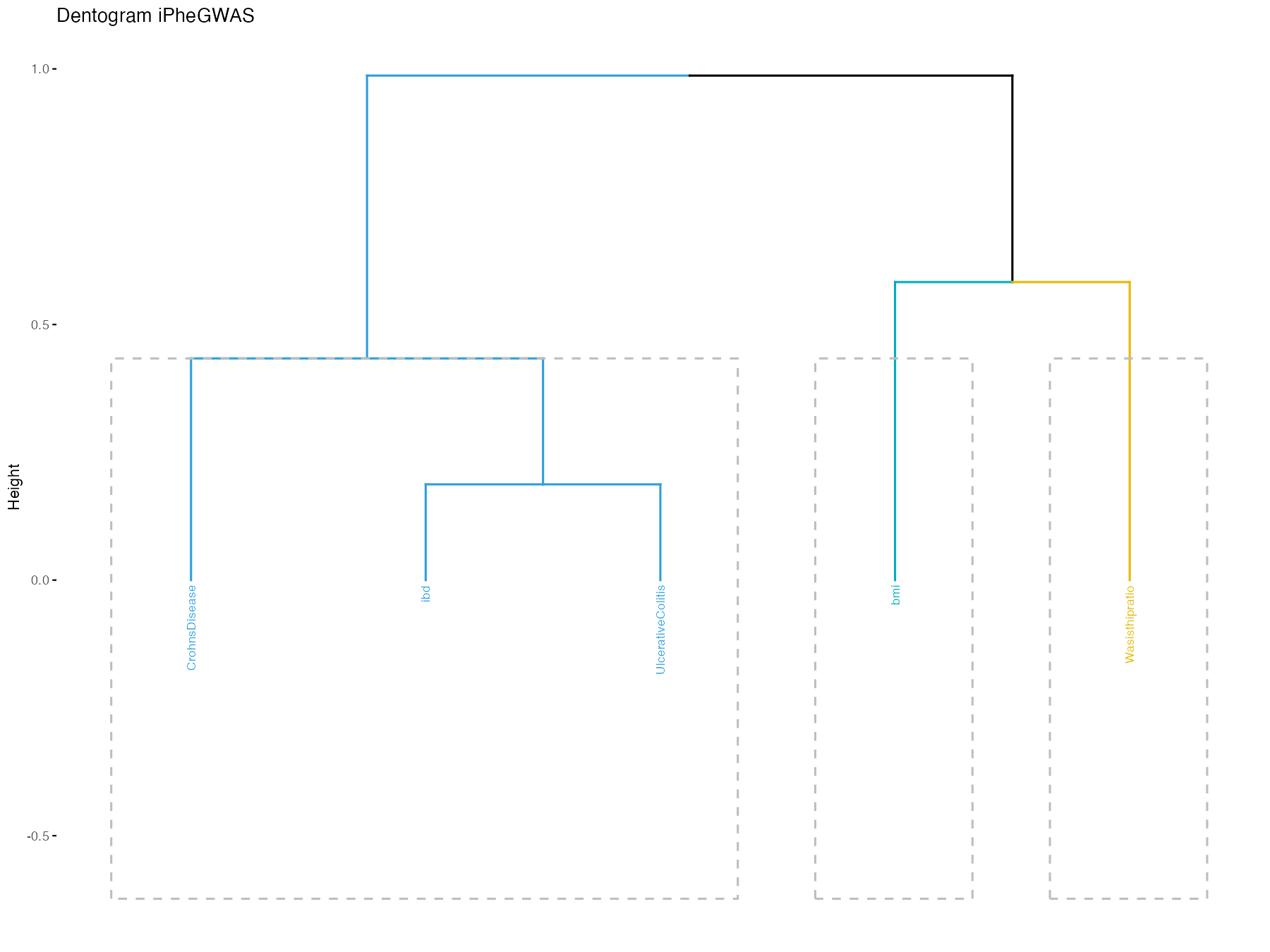
We can use iphegwas module in iPheGWAS package to
determine the genetic similarity between the traits. If we pass the
argument dentogram = TRUE, it will give a dentogram that is
ordered based on the genetic similarity and give further insights to
it’s genetic architecture (for more details checkout paper).
iphegwas(pathname = pathname, dentogram = TRUE)
Passing it without dentogram = TRUE will return ordered
traits. This is useful to pass to the PheGWAS module to order similar
traits in the PheGWAS landscape.
iphegwas(pathname = pathname)
#> [1] "CrohnsDisease"     "ibd"               "UlcerativeColitis"
#> [4] "bmi"               "Wasisthipratio"
Mode 2
head(ibd, 3)
#>    CHR     BP       rsid A1 A2    beta     se P.value
#> 1:   1 721290 rs12565286  c  g  0.0949 0.0408 0.02005
#> 2:   1 752566  rs3094315  a  g -0.0399 0.0193 0.03921
#> 3:   1 752721  rs3131972  a  g  0.0388 0.0194 0.04564
head(bmi, 3)
#>    CHR        BP       rsid A1 A2    beta     se P.value
#> 1:  12 126890980  rs1000000  G  A  0.0001 0.0044 0.98190
#> 2:   4  21618674 rs10000010  T  C -0.0029 0.0030 0.33740
#> 3:   4   1357325 rs10000012  G  C -0.0095 0.0054 0.07853
head(Wasisthipratio, 3)
#>    CHR       BP      rsid A1 A2  beta     se P.value
#> 1:  10 94471975 rs2497311  T  C 0.023 0.0059   1e-04
#> 2:  15 70765255 rs7178130  A  G 0.017 0.0044   1e-04
#> 3:   2 66615915 rs7603236  C  T 0.016 0.0042   1e-04
head(CrohnsDisease, 3)
#>    CHR     BP      rsid A1 A2    beta     se P.value
#> 1:   1 752566 rs3094315  a  g -0.0558 0.0253 0.02774
#> 2:   1 752721 rs3131972  a  g  0.0549 0.0255 0.03149
#> 3:   1 754182 rs3131969  a  g  0.0343 0.0268 0.19940
head(UlcerativeColitis, 3)
#>    CHR     BP       rsid A1 A2    beta     se P.value
#> 1:   1 721290 rs12565286  c  g  0.0575 0.0483  0.2336
#> 2:   1 752566  rs3094315  a  g -0.0299 0.0241  0.2156
#> 3:   1 752721  rs3131972  a  g  0.0321 0.0242  0.1861
## Bringing all package data to the environment
ibd <- ibd
bmi <- bmi
Wasisthipratio <- Wasisthipratio
CrohnsDisease <- CrohnsDisease
UlcerativeColitis <- UlcerativeColitis
Generating dentrograms
phenos <- c("ibd", "bmi", "CrohnsDisease", "UlcerativeColitis", "Wasisthipratio")
iphegwas(phenos, dentogram = TRUE)
iphegwas(phenos)
#> [1] "CrohnsDisease"     "ibd"               "UlcerativeColitis"
#> [4] "bmi"               "Wasisthipratio"
Integration with PheGWAS
The ordering of the PheGWAS landscape is based on the order in which the user passed the phenotypes. So the order here is meaningless, and when dealing with many phenotypes, it is often the case that we would like to group the traits based on their genetic similarity for further investigation on genetic architecture and the correlation drivers from the landscape.
yy <- fastprocessphegwas(phenos)Once the processing is done, pass the dataframe that you got from
fastprocessphegwas to landscapefast to see the
landscape; Here, the landscape orders are in the order that we are
passing the phenos.
print(phenos)
#> [1] "ibd"               "bmi"               "CrohnsDisease"
#> [4] "UlcerativeColitis" "Wasisthipratio"
landscapefast(yy, sliceval = 7, phenos = phenos)
#> [1] "Processing for the entire chromosome"
If you want to order the traits in the landscape based on genetic similarity, then you pass the order that you get from the iphegwas module.
landscapefast(yy, sliceval = 7, phenos = iphegwas(phenos))
#> [1] "Processing for the entire chromosome"
Using ldsc module
Often our users use the iphegwas modules to get insights on all the traits quickly, so they can pick the traits they are interested in and pass those traits to the LDSC module for its genetic correlation values. To develop this R module ( ldscmod ) , we used LDSC python modules - thanks to the LDSC team.
You can use the ldscmod to calculate;
- Genetic correlation plot
- You also get a
correlationmatrixin your global environment that you can use later. Ifcorrelationmatrixexist in your global environment thenldscmodwon’t recalculate the rg, but you can use ldscmod withdentogram = TRUEandplot = TRUE. - Ordered traits based on the LDSC
- Dendrogram based on LDSC
You need to pass the pathname and ldscpath.
The path name is the absolute path to the folder containing the summary
statistics for which you want to find the genetic correlation. You must
have only summary statistics in this folder, or else you will get an
error. All the additional files that LDSC generates will also be put
into the location pathname for later reference if you are
interested in looking at those files for additional metrics that LDSC
provides.
pathname <- system.file("extdata", "samplesummary", package = "iphegwas")
ldscpath <- system.file("extdata", "ldsc", package = "iphegwas")
Using ldscmod to get the genetic correlation plot (using LDSC).
ldscmod(pathname, ldscpath, plot = TRUE)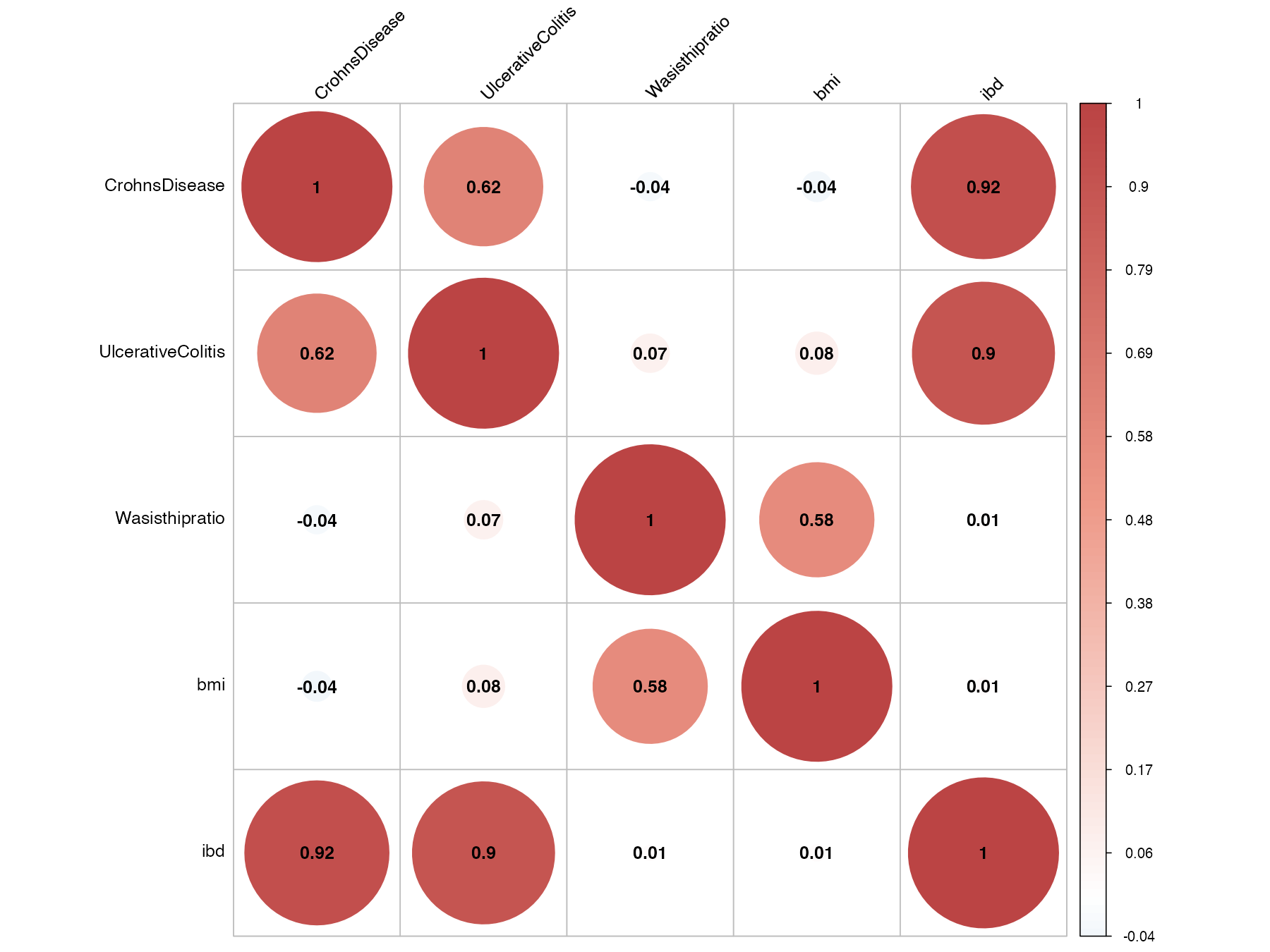
Using ldscmod to examine the dendrograms (using LDSC).
ldscmod(pathname, ldscpath, dentogram = TRUE)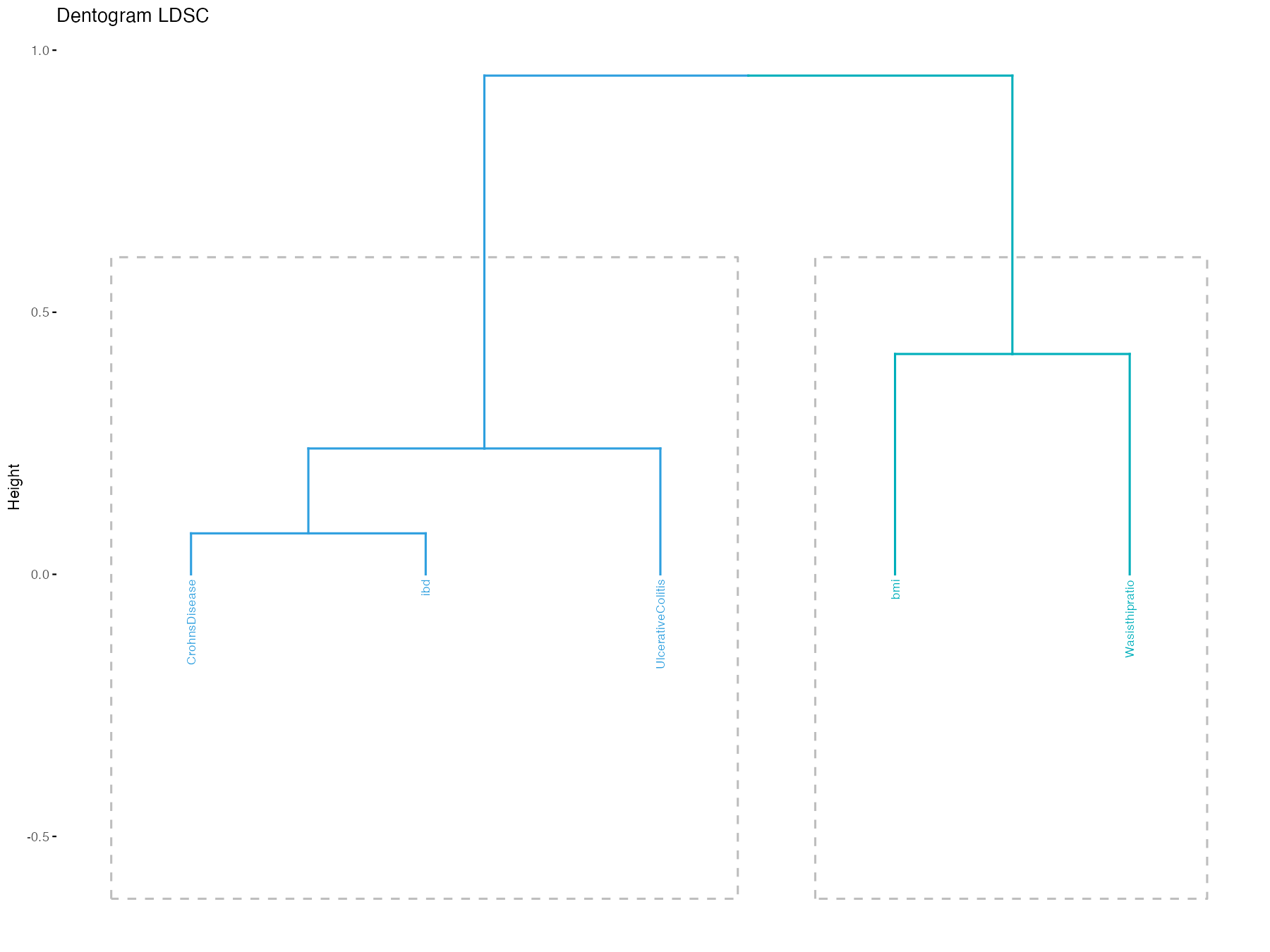
If you want to order the traits in the landscape based on the genetic correlation from LDSC, then you pass the order what you get from the ldsc module.
landscapefast(yy, sliceval = 7, phenos = ldscmod(pathname, ldscpath))
#> [1] "Processing for the entire chromosome"
PheGWAS features
In addition to the heuristic approach that we developed, all the functionalities outlined in the PheGWAS are also available in iphegwas package. Considering performance in mind, the entire codebase is rewritten, and you will notice that the iphegwas package is faster than the PheGWAS package. Adding here the code from the PheGWAS vignette.
Following processed summary data are from the lipid consortium:
head(hdl, 3)
#>   CHR        BP       rsid A1 A2   beta     se P.value
#> 1   7  92383888       rs10  c  a 0.0051 0.0142  0.7646
#> 2  12 126890980  rs1000000  g  a 0.0073 0.0057  0.3375
#> 3   4  21618674 rs10000010  t  c 0.0049 0.0034  0.2546
#>                                                            gene
#> 1                                                          CDK6
#> 2 RP4-809F18.1;RP4-809F18.2;RP5-944M2.1;RP5-944M2.2;RP5-944M2.3
#> 3                            KCNIP4;RP11-556G22.1;RP11-556G22.3
head(ldl, 3)
#>   CHR        BP       rsid A1 A2   beta     se P.value
#> 1   7  92383888       rs10  a  c 0.0317 0.0151 0.03411
#> 2  12 126890980  rs1000000  a  g 0.0050 0.0062 0.51210
#> 3   4  21618674 rs10000010  t  c 0.0058 0.0036 0.13150
#>                                                            gene
#> 1                                                          CDK6
#> 2 RP4-809F18.1;RP4-809F18.2;RP5-944M2.1;RP5-944M2.2;RP5-944M2.3
#> 3                            KCNIP4;RP11-556G22.1;RP11-556G22.3
head(trig, 3)
#>   CHR        BP       rsid A1 A2   beta     se P.value
#> 1   7  92383888       rs10  a  c 0.0163 0.0137 0.39990
#> 2  12 126890980  rs1000000  a  g 0.0114 0.0056 0.08781
#> 3   4  21618674 rs10000010  t  c 0.0032 0.0033 0.26940
#>                                                            gene
#> 1                                                          CDK6
#> 2 RP4-809F18.1;RP4-809F18.2;RP5-944M2.1;RP5-944M2.2;RP5-944M2.3
#> 3                            KCNIP4;RP11-556G22.1;RP11-556G22.3
head(tchol, 3)
#>   CHR        BP       rsid A1 A2   beta     se P.value
#> 1   7  92383888       rs10  a  c 0.0310 0.0148 0.03129
#> 2  12 126890980  rs1000000  a  g 0.0014 0.0061 0.99050
#> 3   4  21618674 rs10000010  t  c 0.0095 0.0035 0.01953
#>                                                            gene
#> 1                                                          CDK6
#> 2 RP4-809F18.1;RP4-809F18.2;RP5-944M2.1;RP5-944M2.2;RP5-944M2.3
#> 3                            KCNIP4;RP11-556G22.1;RP11-556G22.3
## I am changing the name of the dataframe to something meaningful, as the name
## of the dataframe will be used as phenotype names in the landscape. This also
## bring all package data to the environment.
HDL <- hdl
LDL <- ldl
TRIGS <- trig
TOTALCHOLESTROL <- tchol
Note: The gene column is optional. There is an option to map
genes to rsid if you want this, please set genemap = TRUE
(By default it is set to FALSE). If TRUE it
will take some time as it is using Gene BioMart Module to map genes
internally.
The dataframe’s are passed to processphegwas function as a list of dataframe’s.
phenos <- c("HDL", "LDL", "TRIGS", "TOTALCHOLESTROL")
y <- fastprocessphegwas(phenos)
3D landscape visualization of all the phenotypes across the base pair positions(above a threshold of -log10 (p) 6)
landscapefast(y, sliceval = 10, phenos = phenos)
#> [1] "Processing for the entire chromosome"
3D landscape visualization of chromosome number 19 (above a threshold of -log10 (p) 10)
landscapefast(y, sliceval = 7.5, chromosome = 19, phenos = phenos)
#> [1] "Processing for chromosome 19"
3D landscape visualization of chromosome number 19, gene view active (above a threshold of -log10 (p) 10)
landscapefast(y, sliceval = 7.5, chromosome = 19, geneview = TRUE, phenos = phenos)
#> [1] "Processing for chromosome 19"
#> [1] "GENE View is active"
3D visualization with LD block (for european population) passing externally, parameter to pass LD and also calculate the mutualLD block
landscapefast(y, sliceval = 30, chromosome = 19, calculateLD = TRUE, mutualLD = TRUE,
    phenos = phenos)
#> [1] "Processing for chromosome 19"
#> [1] "Calculating the mutually shared SNP's"